The Similarity of Sound: Spotify Recommendations with Feature Geometry

21 Jun, 2025

In the entertainment & streaming industry today, particularly with OTT and audio streaming platforms, content recommendation engines have become pivotal to their adoption. With time, these engines have evolved to become much more sophisticated by leveraging multiple data points about the users (some feature points are not even revealed as they render competitive advantage). However, the intent of this blog post is to de-mystify 'recommendation engines' and build a vanilla recommender from scratch, using nothing but bare math principles. What are we then solving?

Can we, after learning a user's musical taste, automatically pick a few songs from an unknown playlist which would appeal the most to them?

The good news is: YES, we can!

Getting started: Building the user profile

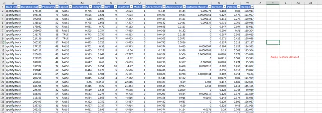
The key ingredient to our success is being able to build a mathematical representation of what our user likes. While as of today, Spotify has banned the export of audio features using their developer APIs (ahh, crap- I know!), we still have a way to export track & feature metadata using Exportify. Each audio track can be quantified into a set number of attributes, such as the 'danceability', or the 'energy', or the 'tempo' (BPM), and the likes. Once exported, the dataset would look somewhat like this.

If we visualize features as points on an N-dimensional space, it becomes easier to apply mathematical principles to compute similarity, such as cosine similarity, Euclidean distance, et cetera. This is exactly what we will apply in this reconstruction. However, before we 'compress' a thousand songs (my liked list is huge!) into my 'preference vector', we will need an aggregation function. Given that certain audio features can be outliers as compared to my general hearing preferences, I would choose median scoring over mean to compute the preference vector. This could of course have different scoring functions for the variety of features.

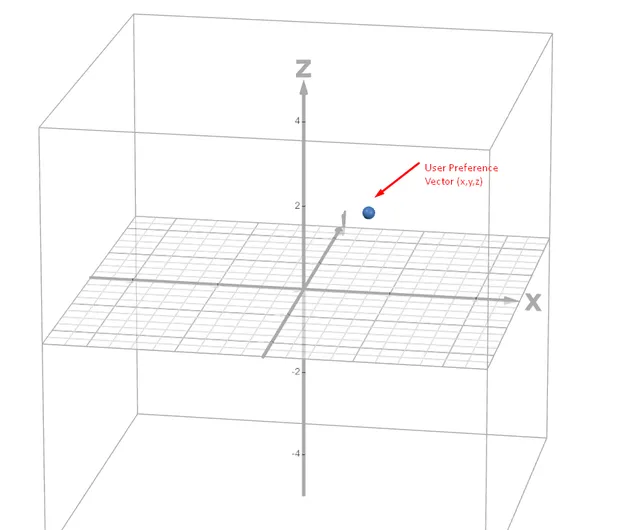
In a 3D space with 3 dimensions, this would appear like this:

Behold the new playlist

Now that a preference vector has been computed in the earlier step, it is time to get rolling! This is the step where we will process the new playlist from which we are to pick our top-N songs for the user. For starters, this is our playlist:

Using the procedure elucidated above, we export the audio track features for the Chill Hits playlist (containing roughly 130 songs), and normalize the features into a Pandas dataframe. This normalization was also done for the preference vector calculation.

import pandas as pd
import numpy as np
from profile_save import preference_vector # Preference vector saved here

def analyze_chill_hits():

    try:
        # Load the chill_hits.csv file
        df = pd.read_csv('chill_hits.csv')
        
        # Define the feature order as specified; VERY IMPORTANT to match with the preference vector
        feature_order = ["Duration (ms)", "Popularity", "Danceability", "Energy", "Key", 
                        "Loudness", "Mode", "Speechiness", "Acousticness", "Instrumentalness", 
                        "Liveness", "Valence", "Tempo"]
        
        features_df = df[feature_order].copy()
    
        features_df_normalized = features_df.copy()
        features_df_normalized["Duration (ms)"] = features_df_normalized["Duration (ms)"] / 60000  # Convert to minutes
        
        # Normalize other features to 0-1 scale where appropriate
        features_df_normalized["Popularity"] = features_df_normalized["Popularity"] / 100
        features_df_normalized["Loudness"] = (features_df_normalized["Loudness"] + 60) / 60  # Normalize loudness (-60 to 0)
        features_df_normalized["Tempo"] = features_df_normalized["Tempo"] / 200  # Normalize tempo (assuming max around 200 BPM)

The next step is to compute the Euclidean distances between the normalized feature vectors for each individual song, to the preference vector already saved in the earlier step. In general, for a N-dimensional space, the Euclidean distance is calculated as follows:

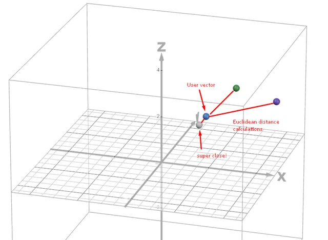
Visually- and for simplicity if we assume the calculation was done on three dimensions alone, it will look somewhat similar to the below plot. Notice how one song is very close to the original preference vector. This is what Euclidean distance calculation does; it figures out the similarity of each individual N-dimensional vector to a centroid vector which is predefined in the space.

The code snippet provided achieves the Euclidean distance computation, and subsequent ordering to pick the top 10 most likely songs to appeal.

distances = []
        for idx, row in features_df_normalized.iterrows():
            song_features = row.values
            distance = np.sqrt(np.sum((song_features - preference_vector_normalized) ** 2))
            distances.append(distance)
        
        # Add distance column to dataframe
        df['distance'] = distances
        
        # Sort by distance (closest first)
        df_sorted = df.sort_values('distance')
        
        print(f"\nTop 10 songs closest to your preference vector:")
        
        for i in range(min(10, len(df_sorted))):
            song = df_sorted.iloc[i]
            print(f"{i+1:2d}. {song['Track Name']:<40} - {song['Artist Name(s)']:<30} (Distance: {song['distance']:.4f})")
        
        return df_sorted

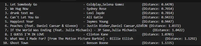
BAM! Now we have the top 10 songs automatically picked up from a subset of over 130 songs, which is quite impressive. This is how it looked like, for me:

Takeaways

Of course, taste is preferential and is actually much more complex to estimate than a simple Euclidean approach demonstrated here. For industry models, there are both statistical and AI/ML approaches to solving the problem at scale. One such approach is the Non-Negative Matrix Factorization, used to identify latent behavioral patterns, and used at places such as Netflix. This is an active field of research, and if you are interested, do check out the wealth of literature available on the subject over the internet.